
Multi linear regression (multivariate linear regression) is the 2nd topic of the regression section of supervised learning.
It is a type of regression that works with the same logic as Simple Linear Regression (univariate linear regression), but with more than 1 variable instead of 1 variable.
Introduction to Multi-Linear Regression
In this section, we will examine why it is used, its formulas, and its differences from univariate regression. If you don’t know univariate linear regression, read this article.
What is Multi-Linear Regression?
multiple linear regression is the analysis to reveal the relationship between the dependent variable and more than 1 independent variable.
Structurally, it is similar to simple linear regression, the only difference is to use more than 1 independent variable instead of looking for a relationship with 1 argument.
In order to apply multiple regression to the data, there should be no multicollinearity between the independent variables.
Multi Linear Regression Formula
Before moving on to the difference between Simple Linear Regression and Multi Linear Regression, let’s examine multi linear regression on the formula.
Y = ß0 + ß1×1 + ß2×2 + ß3×3… + E
In the formula, the variable Y is the dependent variable, the X values are the independent variable and can be used more, and finally, E is the margin of error.
Other signs are the Intercept and the slope for X, respectively. Each variable is multiplied by its intersection and all variables are summed with the intercept.
Multi Linear Regression Vs Simple Linear Regression
The major difference between the two concepts is that one tries to predict the outcome with a single independent variable, while the other uses multiple independent variables.
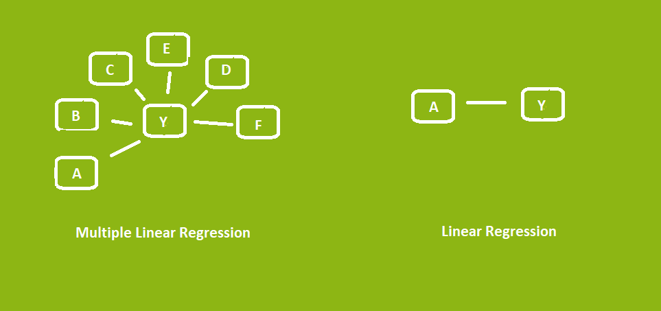
As you can see, one works with a single independent variable and the other with 6 independent variables (the number can be increased).
When Should you Use Which One?
If you have only one independent variable and it is the only factor that affects it, you should use simple linear regression.
Use multi-linear regression if the relationship you want to examine requires more than 1 independent variable, or if it reduces the margin of error of your prediction.
Using too many independent variables does not always reduce your margin of error or improve your prediction, use the right analysis method at the right time.
Dummy Variablies In Multi Linear Regression?
We have come to one of the biggest problems of those who have just started machine learning. A dummy variable can be defined as another variable that expresses a variable.
So what’s the point of this, you might be saying. working with too much data on your machine (I mean empty and useless data) bad affects performance, estimation, and steals your time.
Getting rid of these redundant variables (dummy variables) is actually very easy, mostly if you notice them as soon as you look at the dataset.
Example Dummy Variable
In this section, we will examine a dataset with a sample dummy variable, then we will look at what to do for this dummy variable.

As can be seen in the picture above, an encode was made on a categorical data and converted to numerical data, and also 2 columns were created.
Data in 3 columns are used to the same thing. Divorce and marital status other than the married column must be removed.
Note: Some machine learning algorithms have been immune to a dummy variable trap.
Creating Multi Linear Regression With Python
Before starting this chapter, congratulations! You have finished all the theoretical part and are now ready to create Multi Linear Regression analysis on Python.
In this section, the regression will be created with scikit-learn, and a little knowledge of NumPy and Pandas is required.
You can Download the Dataset Here!
The dataset we will use includes heart statistics and age data. Our main purpose here is to estimate the age of the person who came to the control with heart data.
import numpy as np
import pandas as pd

data = pd.read_csv("Dataset.csv")
data.head(5)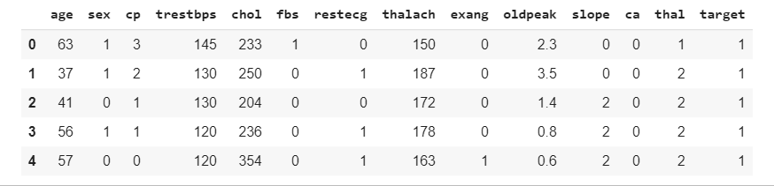
Since there are no null values in the dataset, we do not need to clean the data. If you want to learn how to clean the data, read this article.
# For splitting Dataset
from sklearn.model_selection import train_test_split as tts

X = data.drop("age" , axis = 1)
Y = data.age

x_train , x_test , y_train , y_test = tts(X , Y , test_size = 0.3)
Setting the data to 30% as the test size will often increase the accuracy of the prediction but you can keep it at 20%.
from sklearn.linear_model import LinearRegression

reg = LinearRegression()
reg.fit(x_train,y_train)
The training process of the model is complete, finally, we will generate the predictions and compare these predictions with y_test and examine the error rates.
pred = reg.predict(x_test)
predDf = pd.DataFrame(pred,columns= ["Prediction"])
To make it easier to review later, I converted it to DataFrame, so you can make more comfortable comparisons by converting it.
CompareDf = pd.concat([predDf , y_test])
CompareDf.head(5)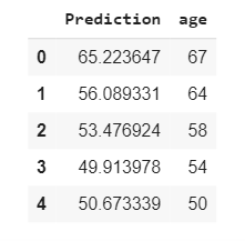
The results look pretty good, now let’s examine the performance of the prediction. The performance will be measured with r2_score, mean_absolute_error, and mean_squared_error.
r2_score: 0.2892470
mean_absolute_error: 6.02
mean_squared_error: 7.268
You can find all functions in sklearn.metrics and you can test your own analysis. Thank you very much for reading