In this article, we will do a study on Python about how to explore datasets, organize your datasets, increase the functionality of datasets.
Exploratory data analysis, or EDA for short, is an application that data scientists use before embarking on a project. Data scientist uses this app to explore and manipulate dataset.
The dataset to be used here will be kept simple and plain for training purposes. You can use the information you have learned here on real datasets. Click to access the dataset.
Introduction
Exploratory data analysis is a method used to explore the data set, in this section, the data set is examined and organized, and most importantly, data cleaning is performed.
Generally, all the results obtained are summarized with data visualization tools.
Installing Required Libraries
There are Python libraries required for exploratory data analysis: pandas, NumPy, seaborn, matplotlib libraries.
pip install pandas
pip install numpy
pip install seaborn
pip install matplotlib
Let’s import these libraries at the beginning of your Python file and start exploratory data analysis.
import pandas as pd
import numpy as np
import seaborn as sb
import matplotlib.pyplot as plt
Explore Dataset
In this section we will integrate the datasets into the project, and use a few features of the pandas library to explore the dataset.
data = pd.read_csv("data.csv")

# Show first 2-row
data.head(2)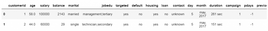
There are only 3 columns we need here, we will separate these columns after the review section, now let’s learn about the other features of the data set.
# For More Information
data.describe()

# It shows null variable and data types
data.info()
Removing Irrelevant Columns
We said that there are 3 columns that are suitable for this analysis. The important point here is that the columns we think are irrelevant may not be irrelevant for your analysis.
This analysis is done to see how age and salary variables affect the duration in the market, so irrelevant columns may change according to the analysis.
# Select column with iloc
data = data.iloc[: , [1,2,13]]
The purpose of this method is to get all rows of columns 1, 2, and 13 and save them as dataset. Now let’s use the drop function.
# Delete columns without 3 columns
data = data.drop(["Column"],axis = 1)
data.head(10)
It can be tiring to enter column names one by one in the list, so using iloc is more efficient. The axis is used to select whether to operate on a column or row.
Converting Categorical Data
This section has been added as it will affect other sections. Not all datasets contain numeric data. Let’s learn how to convert categorical data to numeric data.
To convert the duration value on a time basis to a numeric structure, all it takes is to remove the sec and min statements and convert them all to seconds.
x = 0
for i in data.iloc[: , 2]:

 if "sec" in i:
  iData = i.replace("sec" , "")
  data.iloc[x,2] = float(iData)

 if "min" in i:
  iData = i.replace("min" , "")
  iData = float(data)
  iData *= 60
  data.iloc[x, 2] = iData

 x += 1
How the code works: if there is sec or min in the data, these expressions are deleted and only the numeric part is left, then if data has min, it is multiplied by 60 and converted to seconds.
Data Cleaning
In this section, we will fix the problems that may affect the analysis such as incorrect data and empty data that may occur on the data set.
Dropping Duplicate Rows
First of all, we need to check if there are duplicate rows on the data set, for this we will use the shape and count functions.
# Total number of rows and columns
dataset.shape

# Number of rows per columns
dataset.count()
age 45191
salary 45211
duration 45211
dtype: int64In this data set, which has more than 40,000 rows, some data may be the same, cleaning this data will increase both our performance and efficiency.
We have a function to find duplicate data, but if you want, you can also develop your own function. It is very simple to do.
# select just duplicated rows
copy = data[data.duplicated()]
copy.count()
age 5629
salary 5629
duration 5629
dtype: int645629 rows with the same data were found in the total dataset, this is a large number, we can perform faster processing by deleting this data from the dataset.
# Delete duplicated
data = data.drop_duplicates()
data.count()
age 39562
salary 39582
duration 39582
dtype: int64Cleaning Dataset From Null Values
Null values are structures that can cause problems for many algorithms and analysis. Clearing the data set from them allows us to get more accurate results.
We can use 3 different ways to do this job. In this section, we will delete rows containing null data. Read this article to learn about other methods.
# Lists columns with missing data
print(data.isnull().sum())
age 20
salary 0
duration 0
dtype: int64We are missing 20 data in the Age column. We will analyze approximately 39000 people, so 20 lines will not make a big impact on the program.
Important Note: it may vary from project to project, you can use other methods if the data is important to your analysis.
data = data.dropna()
print(data.isnull().sum())
age 0
salary 0
duration 0
dtype: int64Outliers Cleaning
Deleting outliers usually works well in the project, but it’s more useful to delete when the values you’re going to delete are too far from the mean.
Not every data is an outlier and every outlier should not be deleted, in this section, we will identify and delete outliers with visualization techniques.
sb.boxplot(data["age"])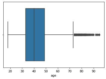
All values out of the box are outliers. Let’s delete the rows in this value range. We will not use the boxplot method for other columns.
# Reset Index Name
data = data.reset_index(drop=True)
The above command will reset the index order corrupted by the columns we have deleted so far. It will work when finding outliers data.
count = 0
deletedcount = 0

for i in data["age"]:
 if i > 75:
  deletedcount += 1
  data = data.drop(count)

 count += 1

print(deletedcount)
This code we wrote will detect the data in the outlier range and delete it from the dataset, you can turn it into a function and save it for using later.
sb.boxplot(data["age"])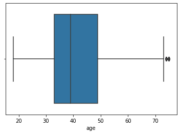
A few outliers in between shouldn’t be a problem, but as you can see we’ve managed to lower the odds quite a bit. You can print the count variable to see how much data has been deleted.
Do you remember, we converted the duration column to a numeric structure, so we can use a visualization tool on it too.
sb.boxplot(data.iloc[: , 2])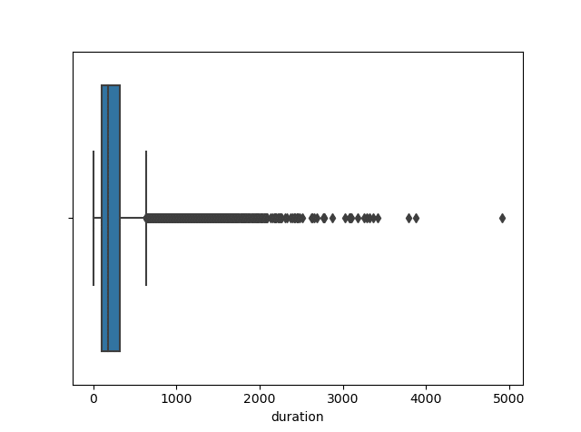
There may seem to be many outliers, but due to the nature of the data, we only need to clean up values above 2000.
we can use the previous function for deletion, with a few edits the previous function will be very useful and practical.
count = 0
deletedcount = 0

for i in data.iloc[: , 2]:
 if i > 1250:
  deletedcount += 1
  data = data.drop(count)

 count += 1

plt.plot()

sb.boxplot(data.iloc[: , 2])

plt.show()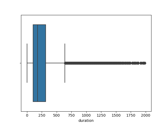
You can edit and manipulate the outliers here as you wish, but it is better to delete data that is well above the average in this way.
Data Analysis – Visualization Data
We discovered our data, cleaned it, organized it, and finally, it was ready for analysis and we can visualize data to report it.
plt.plot()

plt.hist(dataset.age,
         edgecolor='black',
         linewidth=1.2,
         bins = 20)

plt.title("Age Histogram")

plt.show()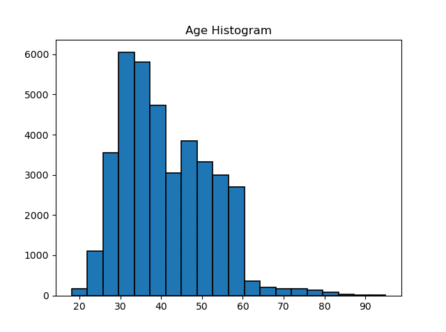
According to the histogram, it is seen that individuals between the ages of 30 and 60 visit the market. Now let’s compare the age data with the duration data with scatter plots.
plt.plot()

plt.scatter(dataset.age,
            dataset.duration,
            s = 0.7,
            color = "red")

plt.title("Age & Duration")

plt.show()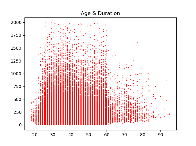
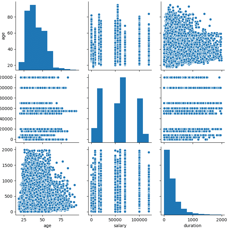
Now we can use the pair plot to make a general visualization, the visualization and reporting tools to be used here may vary depending on the purpose.
Pair plot is a type of multi-chart provided by the seaborn library and is useful for analyzing multiple values.
plt.plot()

sb.pairplot(data, vars=["Age","Salary","Duration"])

plt.show()