
Simple linear regression (univariate regression) it is a subtopic of Supervised Learning, which is used for prediction algorithms.
This article will explain the working logic in a simple way and show you how to use Univariate regression in Python.
Introduction to Simple Linear Regression
First, let’s talk about the regression in Supervised learning, which is a more general definition, then let’s look at linear regression and then univariate regression.
What is Regression?
Regression in supervised learning is a learning method we use to predict an outcome. It has sub-fields such as Linear regression and Polynomial regression.
What is Linear Regression?
Linear regression is a statistical method that examines the linear relationship between two or more variables.
Linear regression is used to find the best fit straight line or hyperplane for a set of points. In other words, linear regression establishes a relationship between the dependent variable (Y) and one or more independent variables (X) using the best fit straight line (regression line).
What is Simple Linear Regression?
There are two types of linear regression, the first is simple linear regression (univariate regression) and second is multiple linear regression with 2 or more independent variables.

As seen in the above visualization, simple linear regression is on a 2D plane while Multiple linear regression is on a 3D plane.
Simple Linear Regression Formula
Another thing we need to learn before we get into practice is the simple linear regression formula. First, I will explain the formula, and then I will show it on a graph.
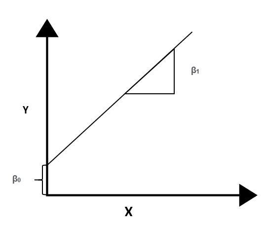
Y = β0 + β1X + ϵ
We use the above formula to explain it simply; Y is the dependent variable, X is the independent variable, β0 where the line intersects the y-axis (regression constant) β1 The slope of the line (regression coefficient) ϵ is the margin of error.
As the independent variable gets larger, the slope will increase and a linear increase will be observed. Therefore, the independent variable is X, while the dependent variable is Y.
We do not need to move on to other formulas, for now, we will focus more on practice than theory.
About Dataset – Weather History Dataset
We will use a dataset that contains almost all the information about the weather in the past. We will examine the relationship between temperature and Apparent Temperature.
We will first analyze and clean these two concepts, which are very suitable for Simple Linear Regression, and then we will create the regression.
An important caveat: Apparent Temperature is calculated together with variables such as wind speed, humidity, but the only temperature will be used in this article because it is a univariate regression.
A multivariate regression can produce more accurate and scientific estimates than this regression, I just use a single variable for this tutorial article.
Simple EDA For Dataset
We will not do a long exploratory analysis, but we will examine important structures such as null data and data formats. If you want to learn more about EDA, read this article.
import pandas as pd
import numpy as np
import seaborn as sb
import matplotlib.pyplot as plt
data = pd.read_csv("weather.csv")
data = data.iloc[: , [3 , 4]]
data.head(5)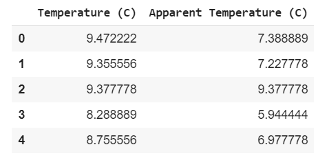
I removed the unnecessary columns from the data set, we will use the data in these two columns for regression, you can examine the whole data set if you want.
data.isna().any()Temperature False
Apparent Temperature False
dtype: boolWe have no empty value, which means no need for data cleaning, what good news! Now let’s check if there are any outliers in the data set, and if there are, let’s clear it.
In addition, you can use the info function to view how much data we have, so you can see how much data you have to work on.
sb.boxplot(data.iloc[: , 0])
sb.boxplot(data.iloc[: , 1])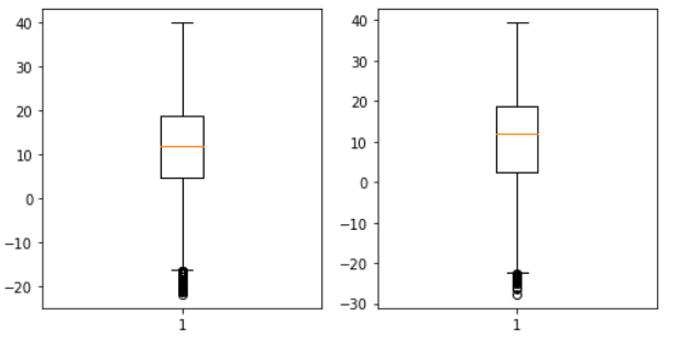
There are outliers slightly below minus value, but I did a little bit of analysis and realized it wouldn’t be right to delete them all, we’ll get rid of a small range.
It’s good for regression to leave some negative data so that our estimates don’t have problems when they get negative values.
count = 0

for i in data.iloc[: , 0]:
  if i < -13:
    data = data.drop(count , 0)

  count += 1

# Reset Index Numbers
data = data.reset_index(drop=True)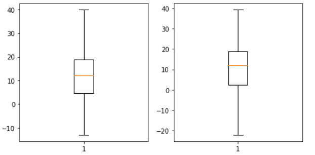
Here I will get rid of duplicate data to reduce unnecessary processing power, we do not need to analyze the same data.
data = data.drop_duplicates()

# Reset Index Numbers
data = data.reset_index(drop=True)
Before: 96328 rows × 2 columns
After: 41556 rows × 2 columnsThe same data doesn’t have a huge impact on the regression, sometimes not at all. It’s often good to clean up.
Simple Linear Regression
I’m starting to build the simple linear regression model, assuming sci-kit is installed. In this section, we will use the data set that we improved in the previous sections.
Before we start, let’s check that the data increases linearly, you can easily do this with a scatter plot.
plt.scatter(data.iloc[0:100,0],
            data.iloc[0:100,1],
            color = "black")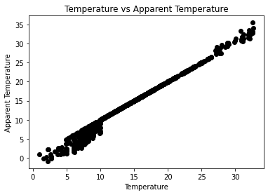
Yes, as it can be seen, it increases linearly, now we can divide the data set into training and test.
from sklearn.model_selection import train_test_split as tts

x = data.iloc[: , 0:1]
y = data.iloc[: , 1:2]

x_train, x_test, y_train, y_test = tts(x, y, test_size=0.3)
The training data is used to train the computer; Both the result and the variable are presented to the computer. There is no result in the test data.
For example, 1 row of the training set; While 32 degrees temperature 35 apparent temperature, there is the only temperature in 1 line of the test set, and the machine predicts the apparent temperature.
Training The Algorithm
The training data provided here also includes the result so that the machine learns how to make decisions then must predict the result itself on the test data.
from sklearn.linear_model import LinearRegression

reg = LinearRegression()
reg.fit(x_train, y_train)
If you didn’t get an error message, congratulations you’ve trained your machine, now let’s test your guesses.
Creating Prediction
predict = reg.predict(x_test)

# Converting data to DataFrame
predictDf = pd.DataFrame(predict, columns = ["Predicted"])

# Merge DataFrames
x = [predictDf, y_test]
result = pd.concat(x,axis=1)

result.head(5)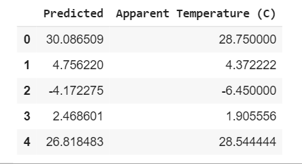
Our margin of error is fine, we have successfully approximated our estimates to reality, if we want to see the margin of error numerically, you can use mean_squared_error.
How the code block here worked; The machine made a prediction with the data it learned and we saved it in a DataFrame and combined the actual and prediction data.
plt.scatter(x_test , y_test)
plt.plot(x_test , predict)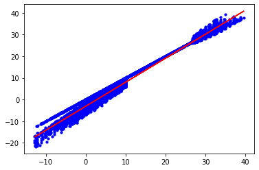
I also visualized it to see how our predictions were shaped. As can be seen, all estimates increase linearly. I hope you liked it and found it useful.