
SQL (Structured Query Language) is one of the most used tools by data scientists, data analysts, and data engineers.
Almost all companies use a SQL-based Database Management System to manage their databases, making SQL an important hiring factor.
No matter how important you are in Python or R, you have to access and edit data, and you can do it with SQL.
What is SQLite?
SQLite is a relational database management system, it is used to manipulate data in tabular form. It is one of the most widely used databases in the world.
SQLite is a disk-based database, so you don’t need a server operation or any other setup other than SQLite, your data will be stored on a disk, not on the server.
The package sqlite3 standard package since Python 2.5 so you don’t need any external library for using SQLite in python.
Importing SQLite3 & Other Required Package
We said we don’t need any package other than SQLite, it’s true we don’t need another package for access SQLite3 but we need a data visualization and analysis package.
import sqlite3 as sql
import pandas as pd
import matplotlib.pyplot as plt

print("Libraries is Launched!")
Pandas is a data manipulation package, matplotlib is a data visualization tool, when we’ll get data on the database we visualize them with matplotlib.
Connecting SQLite Database File
Firstly, we must connect the database for using SQL queries and viewing databases. We connect database file, don’t forget we don’t use the server for SQLite.
# File Path
dbName = "database.sqlite"
source = sql.connect(dbName)

# Shutdown Connection
source.close()
When you work on the database in Python create a variable for the database name, if you change the database name you can edit 1 variable instead of all name values.
SQLite3 database file is supported by different extensions: “.db, .db3, .sqlite3” so if your database file extension is from one of these you can use that file extension.
Create Cursor For Queries
We need an object to execute SQL queries. In the SQLite3, connect class has the execute function to run SQL queries from the script.
cursor = source.cursor()Congratulations, we’ve completed the preparatory steps; now we need a table to hold the data so we create a table, and then we’ll learn how to manipulate data on table.
Creating Table to Store Data
Before creating the data table we need to understand 2 functions in the cursor we’ll use these functions for executing and apply queries.
# Write Queries
cursor.execute()

# Apply Queries
source.commit()

# Close Database
source.close()
Now, we are ready to create the first data table in the database, for creating the database we’ll use create database query in SQL.
createTable =
"""
CREATE TABLE weather
(
  Temp FLOAT,
  WindSpeed INT,
  Humidity FLOAT
);
"""
cursor.execute(query)
source.commit()
Now, we have a table but it’s empty, let’s add some values in the column with the insert query.
addingValues = """
INSERT INTO weather
VALUES(25.5 , 4 , 0.60)
"""

cursor.execute(addingValues)
source.commit()
When using the insert query, enter data according to your column order, data entries are made from left to right.
Now let’s view the data in the table we created, we use the fetchall() function for this, it returns all rows of a query in a list format.
The fetchall() function returns all values, if you want only 1 value, use fetchone(), if you want to return the number of data you specify, use fetchmany().
showQuery = """
SELECT * FROM weather
"""

cursor.execute(showQuery)
source.commit()

print(cursor.fetchall())
1- 25.5|4|0.60As you continue to add data, your data is added from top to bottom, that is, in a 2nd data entry, the data is added to the 2nd row.
Make Automation For Getting Time
We learned how to create a table and how to add values to this table, but maybe you thought this is a very slow process. In this part, we’ll create automation to gain time.
while True:
  q = input("You wanna add: ")

  # Close database & break loop
  if q.lower() == "no":
    source.close()
    break

  # Get Value
  temp = float(input("Temperature: "))
  windSpeed = int(input("Wind Speed: "))
  humidity = float(input("Humidity: "))

  # Create Query
  addingValues = """
  INSERT INTO weather
  VALUES({} , {} , {})
  """

  # Change Curly Brackets to Value
  cursor.execute(addingValues.format(temp , windSpeed , humidity))
  source.commit()

  print("\nRecord Saved!")
Temperature: 27.6
Wind Speed: 17
Humidity: 0.45
Record Saved!You no longer need to write queries over and over to enter data, simply add the variables to the main query.
By storing the automation code in a separate python file, it will be more useful to run it when you want to enter data. You can store other queries in a different file.
Importing CSV File into Database
If you have a ready CSV table instead of creating a new one, you can import the CSV table into SQLite.
You need an SQLite database engine to import a CSV file. You can open this engine via terminal and import your CSV files with this terminal. Download here.
After the installation is complete, you can open the shell where you can operate on the database by typing the following command into your existing terminal.
sqlite3 databaseName.sqlitesqlite3> .mode csv
sqlite3> .import name.csv tbYou must prepare the table you will transfer in advance, prepare your columns according to the number of columns contained in the CSV file you will import.
Manipulating Data on Table
In this section, we will see how to delete and update data to the table with SQL. We will use SQL queries for these operations.
Database Manipulation consists of 3 parts: adding, removing, and updating, we will learn only the 2 operations because we have already seen adding.
Delete Row With Condition
Before we delete or update data, we need to find that data, we can do this with a WHERE query.
delQuery = """
DELETE FROM weather
WHERE Temp = 25.5
"""
cursor.execute(delQuery)
source.commit()
Here, we have requested to delete data containing 25.5 temperatures, but you can make it easier to delete and update by adding an index column to the table.
For example, to delete the 3rd row, you can specify the index instead of the temperature value and delete that row.
Update Data in Row
Instead of deleting the whole row, you can update outdated data. In this example, let’s add an index column to the weather table.
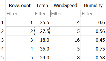
update = """
UPDATE weather
SET Temp = 29.2
WHERE RowCount = 2
"""
cursor.execute(update)
source.commit()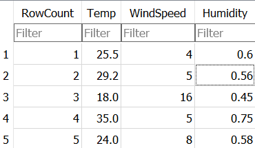
As you can see, you can process faster by giving the number of the row you want to delete or update.
Visualize Weather Data
Let’s see the power of SQLite a little more by using the matplotlib and pandas we installed before with SQLite.
In this section, we will import the weather dataset, which is a ready dataset, to SQLite, manipulate the data and visualize this data with matplotlib.
cursor.execute(
  """
  CREATE TABLE weatherCSV
  (
    location TEXT,
    date TEXT,
    precipitation FLOAT,
    temp_max FLOAT,
    temp_min FLOAT,
    wind FLOAT,
    weather TEXT
  );
  """
)
sqlite3> .mode csv
sqlite3> .import weather.csv weatherCSVWe have a lot of data here so it wouldn’t be convenient to write them all to the screen. We can use LIMIT or fetchmany() to limit this data.
selectQuery = """
SELECT temp_min
FROM weatherCSV
LIMIT 10
"""

cursor.execute(selectQuery)
print(cursor.fetchall())

# You can use this too

selectQuery = """
SELECT temp_min,date
FROM weatherCSV
"""

cursor.execute(selectQuery)
print(cursor.fetchmany(10))
temp_min,date
(5.0,),2012-01-01
(2.8,),2012-01-02
(7.2,),2012-01-03
(5.6,),2012-01-04
(2.8,),2012-01-05
Using LIMIT will be more efficient. Instead of adding all values to an iterator, it adds as much as the value you specify. fetchmany() selects the top 10 of all values.
Now let’s create a DataFrame to visualize, this DataFrame will get the min temperature in the Seattle area from 2012-01-01 to 2012-01-05.
import pandas as pd

df = pd.DataFrame(data = cursor.fetchall(),
                  columns = ["Temp_Min" , "Date"])

# Drop Column Name
df = df.drop(0 , axis = 0)
Temp_Min Date
1 5.0 2012-01-01
2 2.8 2012-01-02
3 7.2 2012-01-03
4 5.6 2012-01-04
5 2.8 2012-01-05Now, we are ready for creating a bar chart with these data. Let’s create a new bar chart in matplotlib.
plt.figure()

plt.bar(df["Date"],
        df["Temp_Min"],
        color = "red",
        width=0.5)

plt.xlabel("Date")
plt.ylabel("Minimum Temp")
plt.title("5-Day Seattle Minimum Temperatures")

plt.show()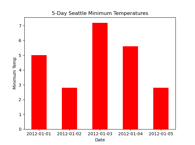
We have given the dates on the X-axis and the lowest temperature of the day on the Y-axis, and you can examine the temperature data in the transition from winter to summer by increasing the number of data.
Or take the summer dates and examine how the highest temperature drops after June 21, or even take the summer temperature average of each year and examine how it changes over the years.
By using the basics here, you can use SQLite effectively in many projects, but a small reminder sqlite3 is API, don’t forget to learn SQL queries for SQLite.