
Computers can solve an event in different ways, we call these ways algorithms, each algorithm works differently from the others and has different processing times.
Since each algorithm takes a different path, its efficiency can vary, and the efficiency of an algorithm is most important to the programmer.
This article is made to show you how to use the commonly used time complexity to measure the efficiency and speed of different algorithms. Good Readings!
Definition of Algorithms
We will measure the efficiency of algorithms, so we need to know what is the definition of algorithms and why we use them in computer science.
The set of steps specifying what operations the computer should perform on the given input is called an algorithm.
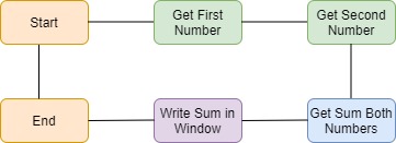
In basic, algorithms are a set of steps for creating output with inputs, for example, if you want a sum is 2 numbers, your algorithm is like in the below diagram.
Now that we know what algorithms are, let’s learn how to measure their efficiency. Let’s start with the first function.
How to Measure Efficiency of Algorithms
With the help of Big O notation, we can calculate how much time an algorithm spends based on the given input.
The running time of an algorithm is expressed in terms of how fast it grows in relation to the input in Big O notation.
In the Big O notation, the input is expressed with (n). For example, if an algorithm’s running time grows according to the input, it is O(n) and if it is a constant value, “n” is ignored and displayed as O(1).
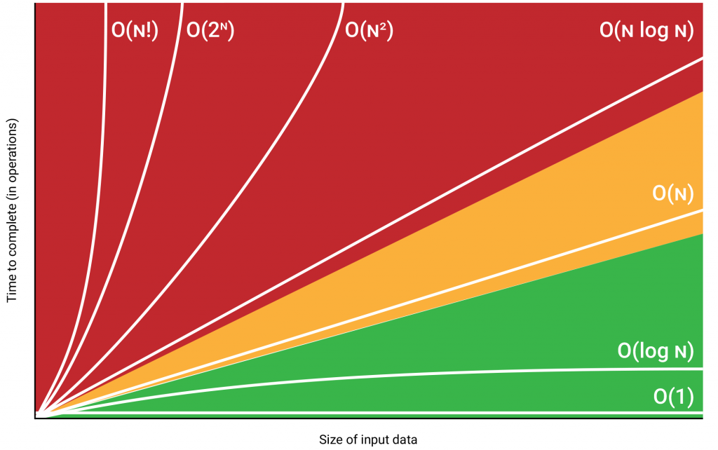
As indicated in the graph, the running time of an algorithm depends on the input and the number of times the algorithm runs (repeats).
While the running time is high in the algorithms in the red area, it is less in the algorithms in the green area.
1 – Constant Time Complexity
The fastest algorithms are included in this class, they do not increase or decrease their running time according to the input. it’s is shown like this O(1).
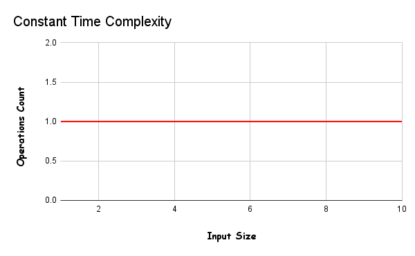
As can be seen, the size of the input (data) does not change the number of operations, and thus the running speed of the algorithms always remains the same.
An example would be using index numbers to access elements of a particular array. No matter how large the data is, a single operation is performed and the runtime does not change.
These algorithms should not contain loops, recursions, or calls to any other non-constant time function in order to remain constant. The run-time of constant-time algorithms does not change: the order of magnitude is always 1.
2 – Linear Time Complexity
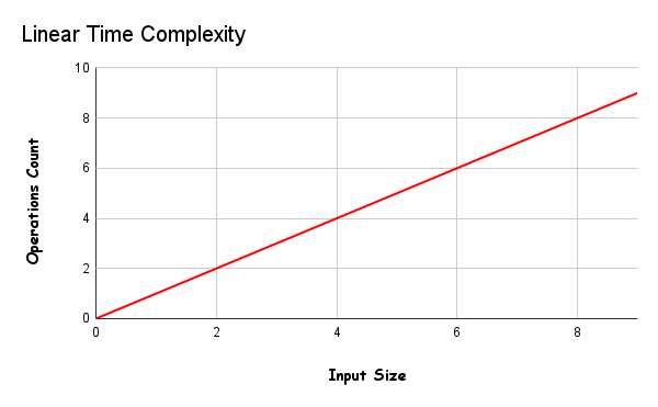
When the time complexity increases proportionally to the size of the input, it is called linear time reciprocity and is denoted by O(n).
These algorithms will process input with the “n” number of operations. That is, the larger the input, the greater the number of operations, which will increase the uptime.
If the algorithm you created works in O(n) time complexity, if it is O(100), the algorithm will run 100 times.
Algorithms such as the radix sorting algorithm, linear search algorithm are included in this class, if your algorithm is returned once in each index, they are also included in this class.
Things like Loops and Recursion must be present in these algorithms, otherwise, it cannot increase the number of input operations, thus not increasing the runtime.
Code Example With Python (Linear Search)
We will create an example of O(n) time complexity in Python so we can grasp exactly how these algorithms work.
The algorithm we will create is a linear search algorithm. With the help of this algorithm, we will search for the data that the user wants in an array.
def linear_search(arr , item):
  for i in range(len(arr)):
      if arr[i] == item:
        return arr[i]

val = linear_search(range(50) , 25)
print("Your Number:" , val)
Since this algorithm tries every element in each index until it finds 25, it works in O(n) time complexity, that is, it performed 25 operations for 25 inputs.
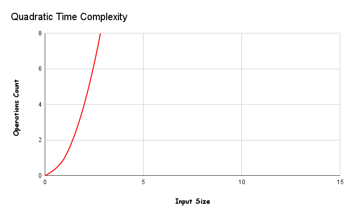
3 – Quadratic Time Complexity
In this type of algorithms, the time it takes to run grows directly proportional to the square of the size of the input. It’s shown is O(n²).
You shouldn’t use these algorithms where there is a lot of input. If you have to use it, separate your input one by one, otherwise you will have trouble.
If you do the linear operation for another linear operation when you use nested loops. Any algorithm that includes a Nested Loop falls into this category.
We don’t recommend using these algorithms if you don’t have enough time and resources, but if you have them and a different algorithm won’t work, you can use this algorithm.
bubble sort algorithm is included in this time complexity, bubble sort algorithm compares a single index with all other indexes. thus resulting in O(n*2) time complexity.
Code Example With Python (Bubble Sort)
Let’s perform the bubble sort algorithm we gave as an example on Python and measure its efficiency.
def bubble(arr):
  l = len(arr)

  for i in range(l):
    for j in range(l - i - 1):
      if arr[j] > arr[j + 1]:
        arr[j], arr[j + 1] = arr[j + 1], arr[j]

    return arr

bubble([3,4,2,6,7,1])
Since the algorithm here tries all the indexes 2 times, O(n^2) time complexity occurs, for example, if 5 inputs are given, the algorithm will run 25 times.
The first loop runs 5 times and the second loop also runs 5 times, 5 x 5 = 5^2, the Big O notation of time complexity is O(n^2).
4 – Exponential Time Complexity
In exponential time algorithms, the growth rate doubles with each addition to the input (n). It’s shown O(2^n).
Algorithms with this time complexity are often used when you don’t know much about the best solution.
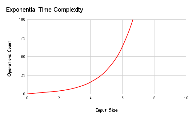
Attention, the range in the operation count axis in the table has been increased. You can see that it takes about 100 times more time than other tables.
Brute-Force algorithms often use this time complexity and initiate a new operation as soon as possible to achieve the correct result.
Exponential time complexity is often seen in Brute-Force algorithms. These algorithms blindly iterate through the entire field of possible solutions to search for one or more solutions that satisfy a condition.
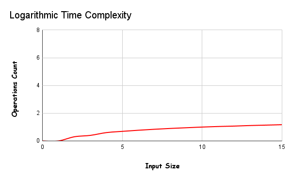
5 – Logarithmic Time Complexity
You are looking for speed, but your algorithm contains loops, the fastest algorithms after constant time algorithms are logarithmic time algorithms. Using these algorithms saves you time.
An algorithm is said to run in logarithmic time if its time execution is proportional to the logarithm of the input size.
This means that instead of increasing the time required to perform each subsequent step, the time is reduced by a magnitude inversely proportional to the input “n”.
Let’s look at the working logic, the algorithms in this category organize the tasks according to the divide and conquer logic, firstly, the tasks are divided into subparts and each piece is solved one by one, saving time.
- Split main input into subparts
- Solve these subproblems recursively.
- Combine the outputs from the subproblems.
An example of this time complexity is binary search, below you can find the working steps of the binary search algorithm.
- Divide the list of your data (vectors, arrays, and so on) in half.
- If the index you have chosen to divide this list is the value you are looking for, end the search.
- If the value you are looking for is less than this index, separate the portion larger than the index.
- If the number you are looking for is greater than this index, delete the part containing the lower values.
- Then check whether the elements in the last list are equal to the searched element one by one.
Congratulations, you have successfully created the fastest search algorithm, the binary search algorithm.
Code Example With Python (Binary Search)
We talked a lot about the Binary Search algorithm, let’s build it on Python.
def search(arr , item):
    mid = len(arr) // 2

    if item == arr[mid]: return arr[mid]

    if arr[mid] > item:
      for i in arr[:mid]:
        if i == item:
          return i

    else:
      for i in arr[mid:]:
        if i == item:
          return i


val = search([1,2,3,4,5,6] , 2)
print(val)
As can be seen, the list was divided into two from the pivot point, then the range of the desired number was determined and only the values in the range were scanned.
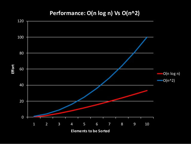
6 – Linearithmic Time Complexity
O(n^2) algorithms generally provide poor efficiency, it is better to use O(n * log(n)) algorithms instead.
These algorithms occur when O(log(n)) algorithms are used together with O(n) algorithms, for example, Merge Sort can be given.
Algorithms with this time complexity divide their work into sub-particles, but O(n) time complexity algorithm is applied on each sub-particle.
Code Example With Python (Quick Sort)
This time complexity can be a bit confusing so I’ll explain further on the code. Let’s start writing the quick sort algorithm.
def quickSort(arr):
 size = len(arr)

 if size <= 1:
   return arr
 else:
   pivot = arr.pop()

 grater,lower = [] , []
 for i in arr:
   if i > pivot:
     grater.append(i)
   else:
     lower.append(i)

 return quickSort(lower) + [pivot] + quickSort(grater)

val = quickSort([1,3,2,4,5])
print(val)
The given input is split into two from the specified pivot point, and the two parts are sorted separately in O(n) time, and finally combined.
Sorting all values in one row requires O(n^2), but if you split it into two parts, the algorithm runs at O(n * log(n)) time complexity.
Summary of the Time Complexity
Let’s make a brief summary of this article, in this section the most important properties of time complexities will be covered.
- O(1) = The running time is fixed, the elements that restart the algorithm, such as loops, recursives, are not found in these algorithms.
- O(n) = The working time increases linearly with the data entered, if you enter 100 data, the number of transactions increases to 100. These algorithms use loops and recursives.
- O(log(n)) = These algorithms are faster than O(n), the input is split in half every cycle, which reduces the number of operations.
- O(n*log(n)) = These algorithms are often confused with O(log(n)), remember that even if the inputs are split in half, there will be recursive in these subsections.
- O(n^2) = Try not to use it, in this algorithm every data on the input is refreshed. In this algorithm, a 5-element string must be run 25 times
- O(2^n) = Use it as a last resort, the performance of these algorithms is very bad. You may encounter it when combination.
Now, there is one last thing left to measure the efficiency of your algorithm, examine your code with the help of a debugger and try to fix the parts that have poor performance.