
The future of the Julia programming language in data science and machine learning looks bright, in this article, we will learn data visualization with Julia.
What is Actually Data Visualization?
Data visualization; is the application of translating data into a visual context, such as a graph, to make it easier for the human brain to understand and gain insight.
In other words, when you make data visualization, the most important thing is to put the data in a way that you can easily understand.
What is Julia and Why We Use?
Julia is a high-level programming language similar to Python and R. Julia is a compiled language, which makes it quicker than Python and R.
Julia was established in 2012, thus it is a new language, yet there are many documents for data science and machine learning.
We chose Julia because it offers more sophisticated data visualization tools and is faster than competitors.
Installing Julia on Local Machine
Let’s start the installation process by installing Julia on your host, you can access Julia’s official site from here, install Julia suitable for your operating system.
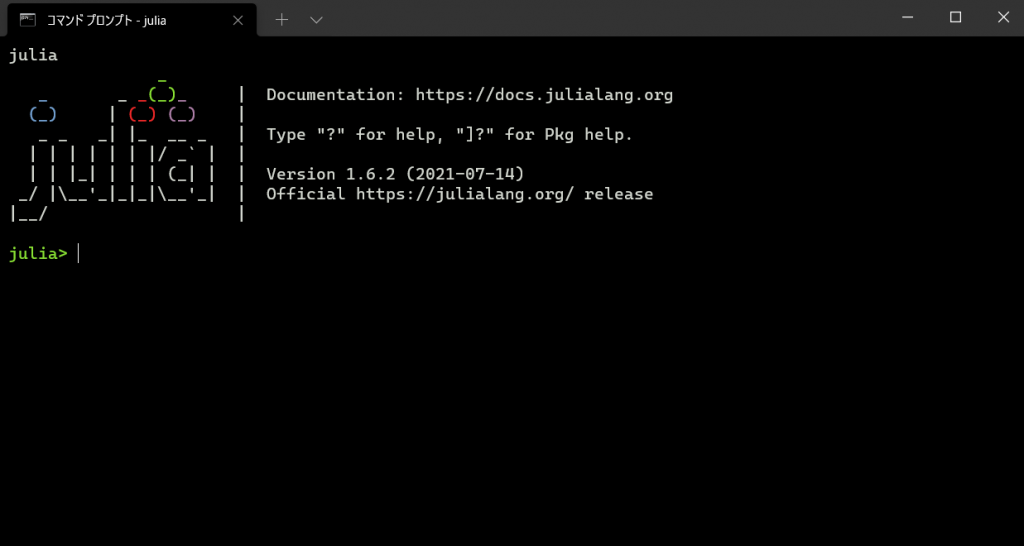
To check that the installation has been completed properly, open a terminal and enter the Julia command, a screen like the one below should appear.
If you are using Visual Studio Code, you can prepare Visual Studio Code for Julia with the help of a few plugins, the following plugins are good for Julia development.
If you are going to use Google Colab, copy the notebook here to the drive and run the commands, then you can write your codes by adding a new code block.
Installing Plots Package
We will use the plots package to create graphs in Julia, you can add this package to Julia with Pkg (Package Manager).
using Pkg
Pkg.add("Plots")
Then you have to import in the project to access all the features of the plots package, you can use the “using” statement for this.
using PlotsLine Chart – Definition Part
Line charts are used to indicate and examine the relationship between 1 dependent and 1 independent variable.
The line chart is formed by combining the spaces between the data in both variables with a line, that is, it can be thought of as a combined version of the data of the scatter chart.
All of the points marked with the marker are data points, when you combine all of these data into a whole (line), a line chart is formed.
Line Chart – Julia Part
Let’s start by creating a simple line chart with Julia. We’ll use a dataset that increases by 2 by 2 for the x-axis, we use a random dataset for the y-axis.
using Random

x_axis = x_axis = [1:1:20;]
y_axis = rand(0:100, 20)
We created two vectors x-axis and the y-axis, the second vector is a vector of randomly selected numbers from the numbers 0 to 100.
The x-axis is a vector that contains all the numbers 1 by 1 from 0 to 20.
using Plots

# Line Chart
plot(x_axis , y_axis)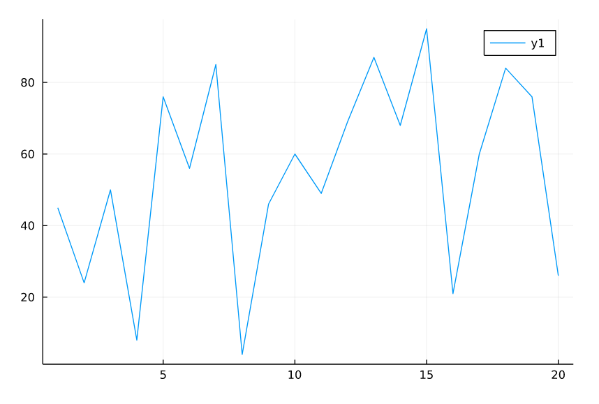
Line Chart with 2 Line
We can increase the number of dependent variables (number of lines) with the plot! function, with the help of this function we can compare 2 dependent variables.
l2 = rand(0:200 , 20)

# Extra Line
plot!(x_axis , l2)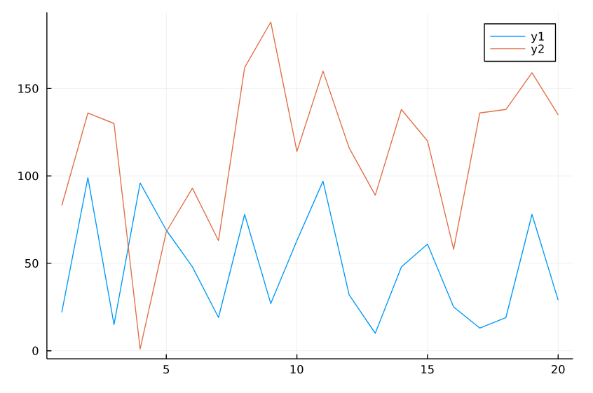
We can customize the line charts a bit more, a perfect chart is the one that is easiest and simplest on the eye.
Customizing the Line Chart
The line chart will be useful in its standard form, but you can make it more beautiful with a few edits.
using Random
using Plots

x_axis = x_axis = [1:1:25;]
y_axis = rand(0:100, 25)
l2 = rand(100:200 , 25)

# Line Chart
plot(x_axis , y_axis, lw = 2 , label = "First" , title = "Simple Line Chart" , color = "tomato1")

# Adding Marker
scatter!(l2 , color = "black", markersize=3 , label = "")

# x and y labels
xlabel!("X axis")
ylabel!("Y axis")

# Extra Line
plot!(x_axis , l2 , label = "Second" , color = "cyan")
We have used the scatter function only to mark the data at the moment, and we will examine it in detail later.
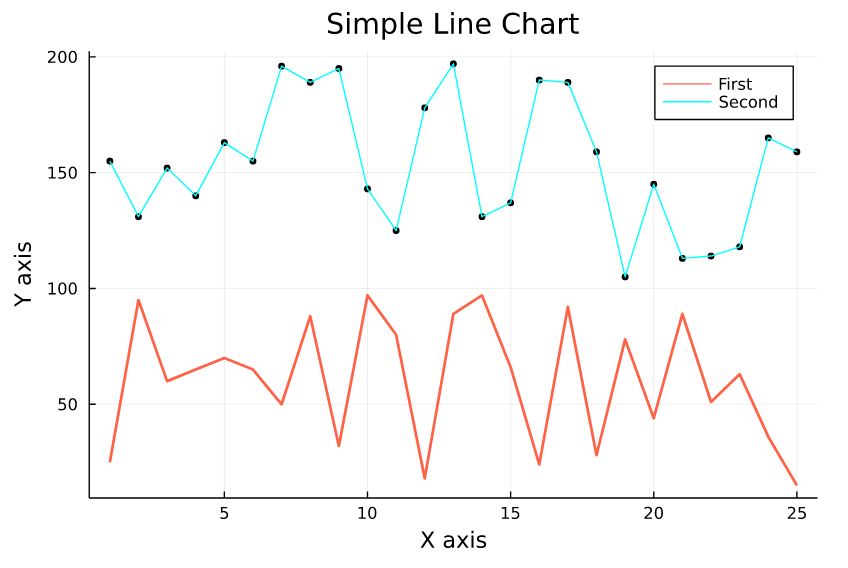
- lw parameter = Used to specify the thickness of the line (default:1)
- label parameter = It is used to change the label of the line.
- title parameter = Allows to give the chart a main title.
- xlabel! and ylabel! = It is used to add labels to the X and Y axes.
You can examine the features of the functions and parameters we used in the list above, now let’s move on to the 2nd graphics technique.
Bar Chart – Definition Part
A bar chart is a way of summarizing a set of categorical data. Each bar is representing the numerical value of its category.
On the X-axis there is the categorical data, on the Y-axis there is the numerical equivalent of these categorical data.
In some cases, categorical data 2 or more bars can be represented by, the purpose here is to compare the bars (data).
Bar Chart – Julia Part
We will not use random values like in the line chart when creating a bar chart, instead, we will use vectors of our own choosing.
In the first example, we will use only one set of data, then we will display the 2 sets of data on a graph.
x_axis = ["x","y","z","k"]
y_axis = [1204,652,978,4622]
In the first example, we’ll compare the monthly earnings data for companies x, y, z, and k on a bar graph.
bar(x_axis , y_axis , bar_width=0.3 , title = "Company Compare Chart" , color = "purple" , legend=:topleft)

xlabel!("Companies")
ylabel!("Sales by Month")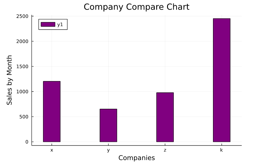
You may have noticed that we are using a few new parameters, let’s examine these parameters, and then we will start working with 2 sets of data.
- legends = We use it to replace the label bar.
- bar_width = used to set the size (thickness) of the bar.
Double Bar Chart
Sometimes, it may be necessary to examine 2 different numerical data on categorical data, in such cases a double bar chart is used.
It is very similar to a bar graph, the only difference is that the number of set of data on the y-axis we used before increases to 2 (the number of set of data may increase)
using StatPlots

x_axis = ["x" , "y" , "z" , "k" , "x" , "y" , "z" , "k"]
sx = repeat(["2020", "2021"], inner = 4)

year2020 = [1000 , 2234 , 3241 , 7653]
year2021 = [5643 , 2345 , 1345 , 8765]

groupedbar(x_axis, [year2020 year2021], group = sx,  color = ["Black" "Orange"])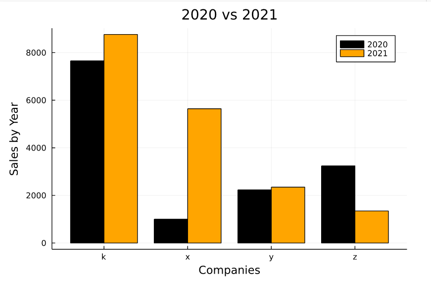
To combine the two bar graphs, the StatPlots package is required. If it is not installed, install it with Pkg (Package Manager).
Histogram – Definition Part
A histogram is a type of chart that is formed by grouping a complex or regular data set on a bar chart.
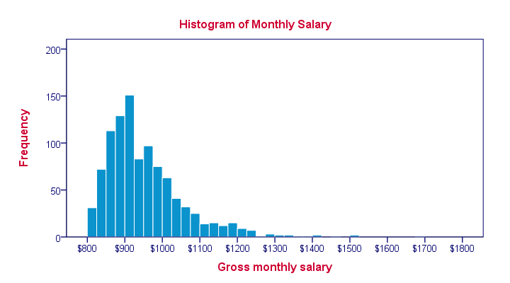
The X-axis is intervals that show the scale of values under which the measurements fall.
The Y-axis shows how many times the values occur within the ranges determined by the X-axis.
Histogram – Julia Part
While creating a histogram, you do not need to prepare any set of data for the y axis. When you prepare the x-axis, the number of times your data is used is automatically determined.
A few collections of sample data you can use for the X-axis: monthly earnings, temperature readings, probability of rain, etc.
using Pkg

Pkg.add("CSV")
Pkg.add("DataFrames")
We will import the data from a CSV file so we install the CSV package to read the CSV files.
We will also be using a DataFrame to store the data so we are adding the DataFrame package to Julia.
using CSV
using DataFrames
using Plots

# Import CSV data
x_axis = DataFrame(CSV.File("temp.csv"))

# Create Histogram
histogram(x_axis[! , 1] , bin = 5 , color = "cyan" , label = "Temp (C)" , title = "Temperature in June")

xlabel!("Temperatures")
ylabel!("Days")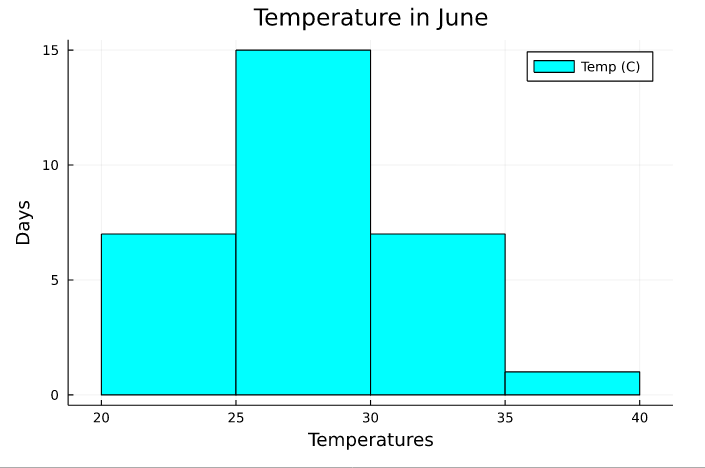
We used the temperature data obtained for 1 month in a histogram, the purpose of this graph is to observe how many days the same temperature is effective.
For example, temperatures between 20 and 25 degrees were observed 7 times in 1 month, and 25 to 30 degrees were observed 15 times in 1 month.
Scatter Chart – Definition Part
Scatter charts are a graphical technique that makes it easy to examine the relationship between dependent and independent variables.
A Scatter Chart, unlike a line chart, uses a collection of points placed using cartesian coordinates to display the values of two variables.
There are two other important terms in scatter charts: outliers and best-fit line. Below you can find simple definitions.
- Outliers: Data that are at a significantly different point from other observations and disrupt the main operation.
- Best fit line: The line formed to be closest to the cartesian points is called. Those that are too far from this line are defined as outliers.
Scatter Chart – Julia Part
You can import a CSV file if you want to work with real data as you saw in the previous section while creating a scatter chart.
using Random

x_axis = 0:100
y_axis = rand(0:100 , 100)
The way data is stored in the same as for a line chart, you can also use the data you use for a line chart in a scatter chart.
using Plots

scatter(x_axis , y_axis , color = "orange" , title = "Scatter Plot")

xlabel!("X axis")
ylabel!("Y axis")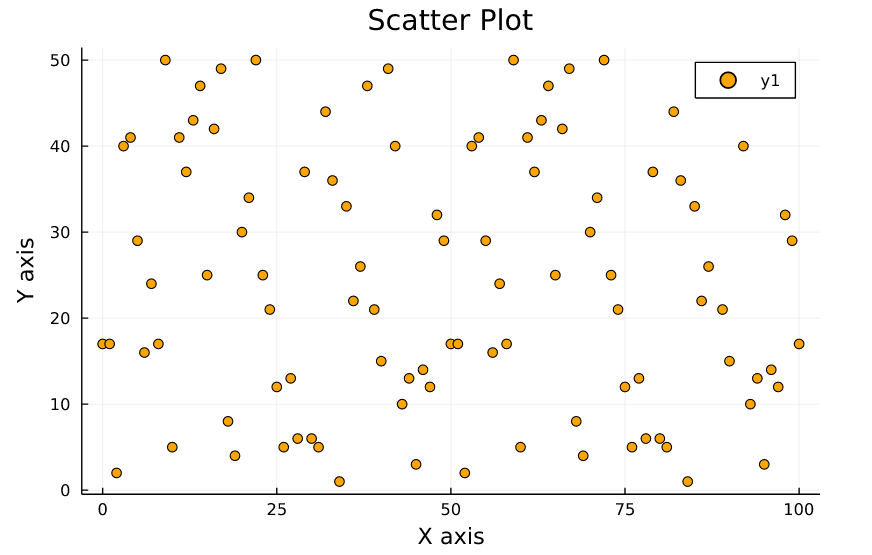
As you can see, a scatterplot is similar to the one above, now let’s prepare a scatterplot created with real data. You can access the dataset from here.
using CSV
using DataFrames
data = DataFrame(CSV.File("data.csv"))
# Get All Row in 2 and 3 column
x_axis = data[! , 2]
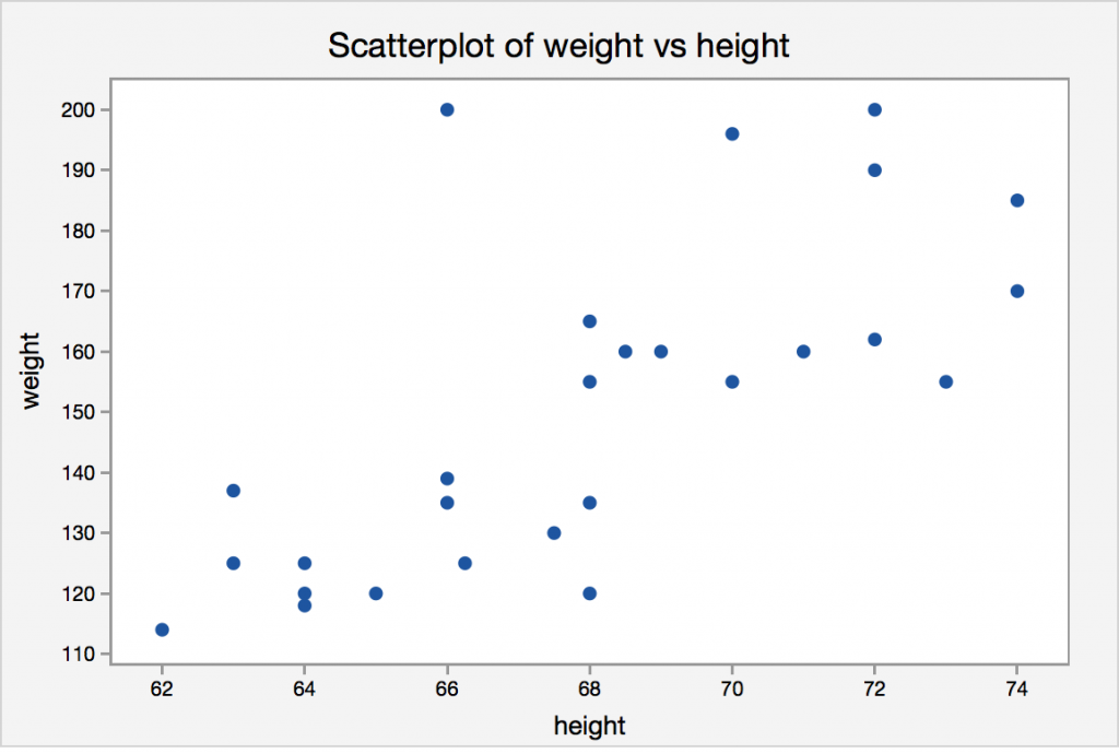
y_axis = data[! , 3]scatter(x_axis[1:1:100] , y_axis[1:1:100] , color = "turquoise" , title = "Weight vs Length", legends=false)
xlabel!("Weight (kg)")
ylabel!("Length (cm)")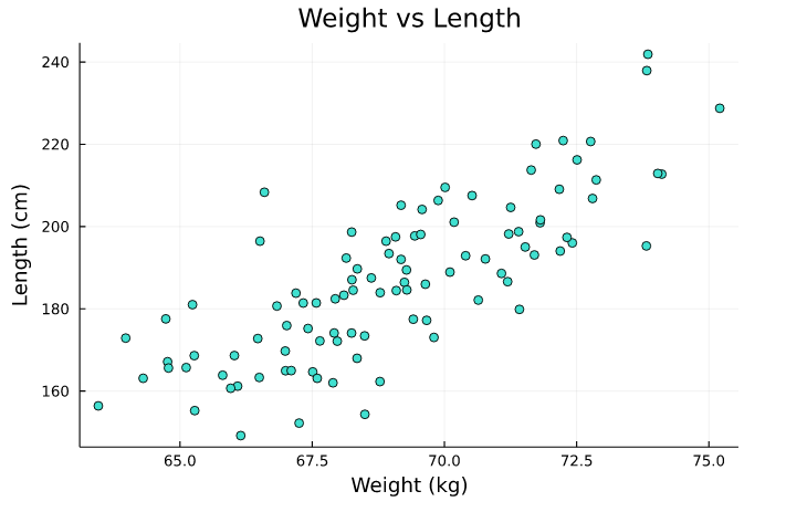
Instead of dumping all the data into a chart, we converted the DataFrame to Vector and set the x_axis and y_axis to hold only 100 data.
Thus, the readability of the chart has increased. A chart holding more than 1000 data will only reduce efficiency. Prefer spreading other data to different charts.
Pie Chart – Technical Part
A Pie Chart is a type of graph that displays data in a circular graph. The pieces of the graph are proportional to the fraction of the whole in each category.
The fraction rate of the categories you enter is adjusted to fill a circle, for example, when you enter 3 different categories, these categories form a circle.
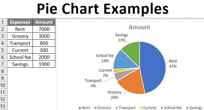
You can find the size of the slice to be covered by the categories with the help of the ratio, the formula is given below. Let’s calculate the area that School Fee’ll occupy on the chart.
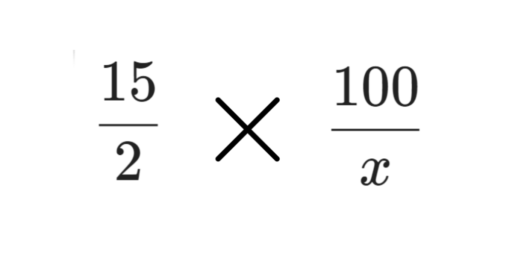
Then you can find the result by doing a cross multiply, solution: 15x = 200 = %13 (approximate value).
Pie Chart – Julia Part
Creating a pie chart is very easy once you know the technical details, let’s start by creating the categories and their values.
January,1200
February,2400
March,3600
April,1800
May,2350
June,1650
We will visualize a data set containing a company’s earnings in the first 6 months (data is fiction) with the help of a pie chart.
using CSV
using DataFrames

data = DataFrame(CSV.File("data.csv"))

# Get All Row in 1 and 2 column
x_axis = data[! , 1]
y_axis = data[! , 2]
pie(x_axis , y_axis , title = "Sales by Month")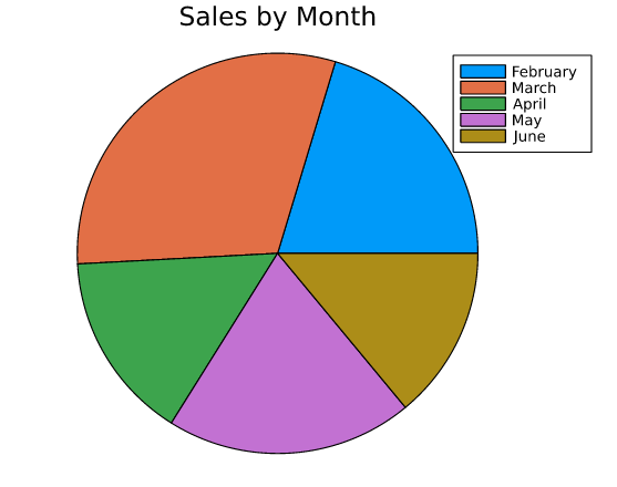
You can calculate the percentage covered by the months with the help of the formula in the definition section.